Overview
The following exercise introduces a variety of useful data analysis utilities in R.
Analysis Routine: Data Import
-
Step 1: To get started with this exercise, direct your R session to a dedicated workshop directory and download into this directory the following sample tables. Then import the files into Excel and save them as tab delimited text files.
Import the tables into R
Import molecular weight table
my_mw <- read.delim(file="MolecularWeight_tair7.xls", header=T, sep="\t")
my_mw[1:2,]
Import subcelluar targeting table
my_target <- read.delim(file="TargetP_analysis_tair7.xls", header=T, sep="\t")
my_target[1:2,]
Online import of molecular weight table
my_mw <- read.delim(file="http://faculty.ucr.edu/~tgirke/Documents/R_BioCond/Samples/MolecularWeight_tair7.xls", header=T, sep="\t")
my_mw[1:2,]
##   Sequence.id Molecular.Weight.Da. Residues
## 1 AT1G08520.1                83285      760
## 2 AT1G08530.1                27015      257
Online import of subcelluar targeting table
my_target <- read.delim(file="http://faculty.ucr.edu/~tgirke/Documents/R_BioCond/Samples/TargetP_analysis_tair7.xls", header=T, sep="\t")
my_target[1:2,]
##      GeneName Loc   cTP   mTP    SP other
## 1 AT1G08520.1   C 0.822 0.137 0.029 0.039
## 2 AT1G08530.1   C 0.817 0.058 0.010 0.100
Merging Data Frames
- Step 2: Assign uniform gene ID column titles
colnames(my_target)[1] <- "ID"
colnames(my_mw)[1] <- "ID"
- Step 3: Merge the two tables based on common ID field
my_mw_target <- merge(my_mw, my_target, by.x="ID", by.y="ID", all.x=T)
- Step 4: Shorten one table before the merge and then remove the non-matching rows (NAs) in the merged file
my_mw_target2a <- merge(my_mw, my_target[1:40,], by.x="ID", by.y="ID", all.x=T)  # To remove non-matching rows, use the argument setting 'all=F'.
my_mw_target2 <- na.omit(my_mw_target2a) # Removes rows containing "NAs" (non-matching rows).
- Homework 3D: How can the merge function in the previous step be executed so that only the common rows among the two data frames are returned? Prove that both methods - the two step version with
na.omitand your method - return identical results. - Homework 3E: Replace all
NAsin the data framemy_mw_target2awith zeros.
Filtering Data
- Step 5: Retrieve all records with a value of greater than 100,000 in ‘MW’ column and ‘C’ value in ‘Loc’ column (targeted to chloroplast).
query <- my_mw_target[my_mw_target[, 2] > 100000 & my_mw_target[, 4] == "C", ]
query[1:4, ]
##              ID Molecular.Weight.Da. Residues Loc   cTP   mTP    SP other
## 219 AT1G02730.1               132588     1181   C 0.972 0.038 0.008 0.045
## 243 AT1G02890.1               136825     1252   C 0.748 0.529 0.011 0.013
## 281 AT1G03160.1               100732      912   C 0.871 0.235 0.011 0.007
## 547 AT1G05380.1               126360     1138   C 0.740 0.099 0.016 0.358
dim(query)
## [1] 170 8
- Homework 3F: How many protein entries in the
my_mw_targetdata frame have a MW of greater then 4,000 and less then 5,000. Subset the data frame accordingly and sort it by MW to check that your result is correct.
String Substitutions
- Step 6: Use a regular expression in a substitute function to generate a separate ID column that lacks the gene model extensions. «label=Exercise 4.7, eval=TRUE, echo=TRUE, keep.source=TRUE»=
my_mw_target3 <- data.frame(loci=gsub("\\..*", "", as.character(my_mw_target[,1]), perl = TRUE), my_mw_target)
my_mw_target3[1:3,1:8]
##        loci          ID Molecular.Weight.Da. Residues Loc  cTP   mTP    SP
## 1 AT1G01010 AT1G01010.1                49426      429   _ 0.10 0.090 0.075
## 2 AT1G01020 AT1G01020.1                28092      245   * 0.01 0.636 0.158
## 3 AT1G01020 AT1G01020.2                21711      191   * 0.01 0.636 0.158
- Homework 3G: Retrieve those rows in
my_mw_target3where the second column contains the following identifiers:c("AT5G52930.1", "AT4G18950.1", "AT1G15385.1", "AT4G36500.1", "AT1G67530.1"). Use the%in%function for this query. As an alternative approach, assign the second column to the row index of the data frame and then perform the same query again using the row index. Explain the difference of the two methods.
Calculations on Data Frames
- Step 7: Count the number of duplicates in the loci column with the
tablefunction and append the result to the data frame with thecbindfunction.
mycounts <- table(my_mw_target3[,1])[my_mw_target3[,1]]
my_mw_target4 <- cbind(my_mw_target3, Freq=mycounts[as.character(my_mw_target3[,1])])
- Step 8: Perform a vectorized devision of columns 3 and 4 (average AA weight per protein)
data.frame(my_mw_target4, avg_AA_WT=(my_mw_target4[,3] / my_mw_target4[,4]))[1:2,5:11]
##   Loc  cTP   mTP    SP other Freq.Var1 Freq.Freq
## 1   _ 0.10 0.090 0.075 0.925 AT1G01010         1
## 2   * 0.01 0.636 0.158 0.448 AT1G01020         2
- Step 9: Calculate for each row the mean and standard deviation across several columns
mymean <- apply(my_mw_target4[,6:9], 1, mean)
mystdev <- apply(my_mw_target4[,6:9], 1, sd, na.rm=TRUE)
data.frame(my_mw_target4, mean=mymean, stdev=mystdev)[1:2,5:12]
##   Loc  cTP   mTP    SP other Freq.Var1 Freq.Freq   mean
## 1   _ 0.10 0.090 0.075 0.925 AT1G01010         1 0.2975
## 2   * 0.01 0.636 0.158 0.448 AT1G01020         2 0.3130
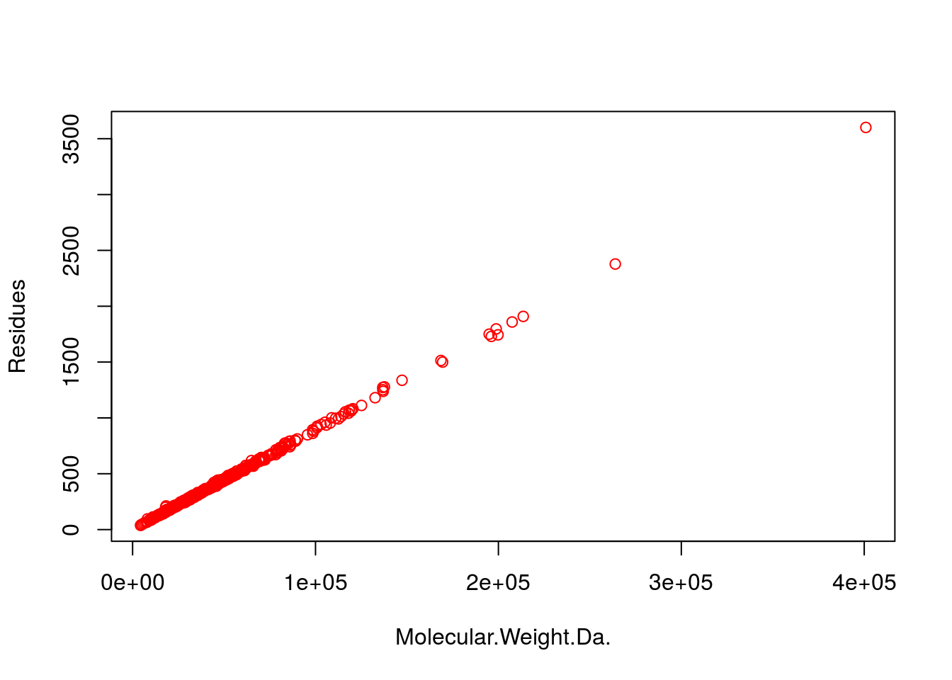
Plotting Example
- Step 10: Generate scatter plot columns: ‘MW’ and ‘Residues’
plot(my_mw_target4[1:500,3:4], col="red")
Export Results and Run Entire Exercise as Script
- Step 11: Write the data frame
my_mw_target4into a tab-delimited text file and inspect it in Excel.
write.table(my_mw_target4, file="my_file.xls", quote=F, sep="\t", col.names = NA)
- Homework 3H: Write all commands from this exercise into an R script named
exerciseRbasics.R, or download it from here. Then execute the script with thesourcefunction like this:source("exerciseRbasics.R"). This will run all commands of this exercise and generate the corresponding output files in the current working directory.
source("exerciseRbasics.R")